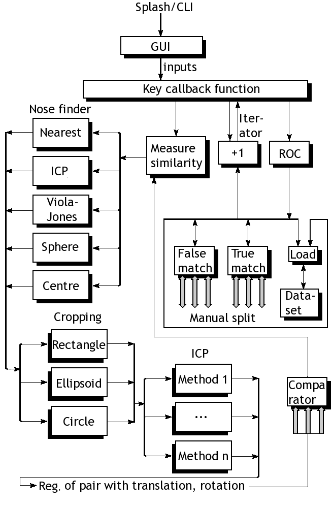
 Depiction of the framework for detection and classification of 3-D data such as faces or internal organs, as well as benchmarking
Summary: Personal take on why software is just symbiosis of maths
This post is a concise summary of something I have been working on (source code will be uploaded at a later date when I tidy everything up). The figure at the top shows a breakdown of our existing framework, which basically depicts a program as a set of black boxes. Each box merely performs mathematical operations on volumetric matrices. It's maths. It can also be specified most precisely using equations (no need for explanation using code or pseudo-code). For the sake of simplicity, the block diagram contains only core components that are used irrespective of the approach tested. The file loaders, for example, are shown separately. They work very well and can elegantly load datasets based on a data selector. With the exception of test sets that are small (remnants of debugging), there are 6 families of data, some grouped in pairs, some grouped by training/target, some our lab's data in isolation, others for FRGC data from NIST. There are also correct and incorrect matches in isolation. These simplify the plotting of ROC curves in a largely streamlined fashion. The goal is the program is to test new metrics that can be used to analyse anything elastic such as tissue. It has uses in cardiac analysis, brains, and even faces (I have dealt with each of these data types). For large quantiles of 3-D data, about 70 GB of face data gets used.
The nose-finding part may as well be treated as a component that provides orientation o a form of segmentation (it can be a face or even an internal organ which we wish to model and perform binary diagnosis on). Depending on the datasets, different methods are used. Commonly, FRGC data is better off interpreted by finding nearest point, excepting noise. For the lab's data, it is preferable to choose the nearest point within a specified region (usually around the centre, no weighting/scoring based on location although that too would work). This can also be done using ICP, as described later (settings inherited from another box/module) or a Viola-Jones approach with face templates for training, although it is only partly implemented so far. Sphere intersection with plane, as per Mian
et al. (with separate slider for radius), is another existing option, but it does not appear to outperform the simpler methods, which work most of the time given some reasonable boundaries (e.g. boundaries to dodge the hair region).
Having identified the tip of the nose correctly, we are cropping out what is left for rigid areas to be isolated. It is quite customisable. Various separation methods and boundary types like circle, ellipsoid, and rectangle have been tested, where circle is the most commonly used one that works in conjunction with binary masks. These come with many sliders and use measurements in X and Y to estimate real physical distances and then factorise pixel-space units, accordingly. There is also a slider for further manual tweaking. And still, it's all maths.
There are some other bits of operation that are worth mentioning; left out from the diagram in order to reduce clutter are smoothers, hole removers, outlier eliminators, and rounding up of values, all of which are optional and very much depend on the data at hand and how it ought to be treated. For instance, FRGC data hardly requires any smoothing. Lab data has offsets that need to be handled systematically depending on the image number. In fact, both datasets do need a lot of branching/forking in the code as their handling and even their size varies (the program is built to handle any image side with any aspect ratio, but for sub-regions to be defined it uses absolute and not relative coordinate inputs).
Then we come to the key part, which actually does more to contribute toward similarity measures. ICP becomes very important in case the initial alignment of the noses is deemed incorrect or the faces are tilted. In practice, assuming the faces are forward-looking and bend neither to the sides or top/bottom, ICP is not supposed to change much. The methods already available are Mian's early ICP method, Mian's most recent ICP method, Raviv's ICP implementation from 2008, and Raviv/Rosman ICP implementation from recent months or years. The program optionally applies translation and optionally it applies the rotation too. In many cases this does not seem necessary as ICP hardly modifies anything substantial.
The model part is not included in the diagram as there are many different things are can be done with a model. PCA, model-building, model assessment, file loaders for models (about 2 gigabytes for some), in addition to more basic measures on which assessment is applied, are basically all sorts of comparators which yield one value for each pair, then proceeding to the plotting of ROC curves (mostly automated following experimental design).
All the above is just mathematics. It can all be described using equations. To patent such stuff would be to claim a monopoly on equations, which means the monopoly covers a wide range (infinite even) of implementations. How can anybody defend the argument that software is not maths? Or that "innovative" software is somehow the exception? If many equations are already patented, how is one supposed to code safely? How can existing methods be enhanced without a violation?

 Depiction of the framework for detection and classification of 3-D data such as faces or internal organs, as well as benchmarking
Comments
Needs Sunlight
2011-05-25 09:42:59
That is why the expression of these ideas is governed by copyright, rather than allowing a blanket monopoly on using the general idea.
Dr. Roy Schestowitz
2011-05-25 10:35:46
Can one patent Newton's Laws to get a monopoly on software/games where gravity and force impacts are simulated (e.g. Angry Birds)? It would be like getting a monopoly on Mother Nature.